Programming

Building a Web Search Engine with Django: A Comprehensive Guide

Building a Web Search Engine with Django: A Comprehensive Guide

Elias Owis

Software Engineer

Introduction:

In today’s digital age, information is abundant and easily accessible online. However, the large volume of data can sometimes make it challenging to find specific information quickly. This is where search engines come to the rescue, helping us sift through the vast ocean of data and locate what we need with just a few keystrokes.

Have you ever wondered how these search engines work under the hood? How do they crawl the web, index web pages, and provide relevant search results? If you’ve ever been curious about building your own web search engine, you’re in the right place.

In this article, we’ll take you on a journey to create a fully functional web search engine using the power of Django, a high-level Python web framework. We’ll leverage my open-source project available on GitHub, called “search_engine_spider” as our starting point. This project provides the essential tools and infrastructure needed to crawl web pages, extract information, and store the results in a database.

Whether you’re an aspiring developer looking to dive into web crawling and search engine development or a seasoned Django enthusiast eager to expand your skill set, this guide has something for you. By the end of this article, you’ll have a solid understanding of how to build a web search engine from scratch, and you’ll be well-equipped to customize it to suit your specific needs.

Let’s embark on this exciting journey to unlock the world of web search engines with Django!

Project Prerequisites:

Before we dive into the nitty-gritty of building our web search engine with Django, let’s ensure we have all the prerequisites in place. To follow along with this tutorial, you’ll need the following:

  • Python 3.x: Django is a Python web framework, so make sure you have Python 3.x installed on your system.
  • Django: our web framework of choice, which will provide the structure for our project.
  • BeautifulSoup: We’ll be using BeautifulSoup to parse web page content.
  • Requests: This library is essential for making HTTP requests to fetch web pages.
  • Database: Decide on the database you want to use. We recommend PostgreSQL if you plan to enable parallel crawling due to its support for concurrent access. SQLite is an option too, but keep in mind that it limits crawling to a sequential process.

What We Will Build:

In this tutorial, we’ll start with a solid foundation – the “Search Engine Spider” available on GitHub. This project provides a pre-built Django application that includes a web crawling utility, a Django management command for initiating the crawling process, and a user-friendly web interface for searching the scraped data.

We will explore how to use the included Spider class to crawl web pages, extract information, and store the results in a database. You’ll also learn how to configure your database settings and decide whether to enable parallel crawling based on your needs.

The web interface we’ll create allows users to enter search queries and retrieve search results from the database. By the end of this tutorial, you’ll have a functioning web search engine that you can customize and expand to suit your specific requirements. Whether you’re interested in web crawling, database management, or building user interfaces with Django, this project will provide valuable insights into each of these areas.

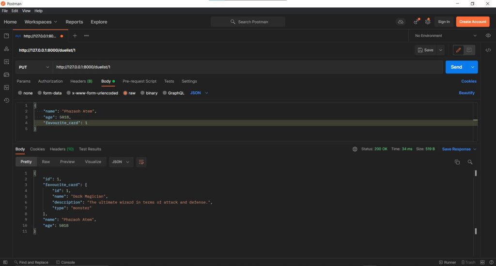
ScrapingResult Model:

The heart of our web search engine project is the ScrapingResult model. This Django model defines the structure in which we store the information we gather during web crawling. Let’s take a closer look at the model’s code and its significance:

class ScrapingResult(models.Model):
    title = models.CharField(max_length=200)
    content = models.TextField()
    url = models.URLField()

    def __str__(self):
        return self.title

  • ScrapingResult is a Django model, and each instance of this model represents a single result obtained from crawling a web page.
  • It has three main fields:
    • title: A CharField which stores the title of the web page, which is typically found within the HTML <title> tag.
    • content: A TextField where we store the text content extracted from the web page. This field captures the textual information from the entire page.
    • url: A URLField that stores the URL of the web page we crawled.

In essence, the ScrapingResult model acts as our structured data store, allowing us to save the titles, content, and URLs of web pages we’ve crawled. This structured storage makes it easy to manage and retrieve the information we need for search functionality and display to users in our web interface.

Understanding Views, Templates, and SearchForm:

In our web search engine project built with Django, Views, Templates, and the SearchForm are used to create a seamless user experience. Let’s break down each of these components:

  • Views: In Django, views are responsible for processing user requests and returning appropriate responses. In our project, we have two key views. The search_page view renders a search form template where users can input their queries. The search_results view handles the search logic, querying the ScrapingResult model to find matching results and rendering them for display. Additionally, this view provides support for AJAX-based pagination, ensuring efficient navigation through search results.
  • Templates: Templates in Django are used to generate HTML dynamically. In our project, we have several templates, including layout.html, search_form.html, search_results.html, and search_result_item.html. layout.html serves as the base template for all pages, providing a consistent structure. search_form.html presents the search input form to users, while search_results.html displays the search results along with pagination. search_result_item.html is a partial template used to format individual search result items. Together, these templates create a user-friendly interface for interacting with the search engine.
  • SearchForm: The SearchForm is a Django form class that handles user input for search queries. It is defined in the code and used in the search_page view. This form ensures that user input is validated, and it simplifies the process of gathering query parameters. It’s a crucial component for user interaction as it enables users to submit their search queries efficiently.

In summary, views manage the logic behind our web pages, templates provide the visual representation, and the SearchForm streamlines user input handling. Together, they form the backbone of our web search engine, delivering a smooth and intuitive search experience to users.

Spider (Crawler):

Certainly, let’s break down the functionality of the Spider class step by step, explaining each part of the code:

class Spider:
    def crawl(self, url, depth, parallel=True):
        try:
            response = requests.get(url)
        except:
            return

        content = BeautifulSoup(response.text, 'lxml')

        try:
            title = content.find('title').text
            page_content = ''
            for tag in content.findAll():
                if hasattr(tag, 'text'):
                    page_content += tag.text.strip().replace('\\n', ' ')
        except:
            return

        ScrapingResult.objects.get_or_create(url=url, defaults={'title': title, 'content': page_content})

  1. The crawl method initiates the crawling process. It takes three parameters:
    • url: The URL to start crawling from.
    • depth: The depth of crawling, determining how many levels of links to follow.
    • parallel: An optional parameter that enables parallel crawling.
  2. Inside the method, it starts by making an HTTP GET request to the provided URL using the requests library. If there’s an issue with the request, it returns early.
  3. It then parses the HTML content of the web page using BeautifulSoup and stores it in the content variable.
  4. The code tries to extract the title and textual content from the web page. It looks for the <title> tag to get the title and iterates through all tags on the page to extract and concatenate their text content.
  5. The extracted title and page_content are used to create a new ScrapingResult instance, which is saved to the database using get_or_create. This method ensures that if the URL already exists in the database, it updates the existing record with the new title and content.
        if depth == 0:
            return

        links = content.findAll('a')

        def crawl_link(link):
            try:
                href = link['href']
                if href.startswith('http'):
                    self.crawl(href, depth - 1)
                else:
                    parsed_url = urlparse(url)
                    protocol = parsed_url.scheme
                    domain = parsed_url.netloc
                    self.crawl(f'{protocol}://{domain}{href}', depth - 1)
            except KeyError:
                pass

        if parallel:
            with ThreadPoolExecutor(max_workers=10) as executor:
                executor.map(crawl_link, links)
        else:
            for link in links:
                crawl_link(link)

  1. Next, the code checks if the specified depth has been reached (depth equals 0). If so, it returns, effectively limiting the depth of the crawling process.
  2. It then extracts all the links (<a> tags) from the current web page and stores them in the links variable.
  3. The crawl_link function is defined to crawl individual links. It extracts the href attribute from the link, and if it starts with “http,” it recursively calls the crawl method for that URL with a reduced depth. If the link is relative, it constructs an absolute URL using the current page’s protocol and domain.
  4. Depending on the parallel flag, the code either processes the links in parallel using a thread pool or sequentially.

In summary, the Spider class crawl method retrieves web pages, extracts their title and content, and stores the results in the ScrapingResult model. It then follows links to other web pages, either in parallel or sequentially, based on the specified depth. This recursive crawling process allows the spider to traverse multiple levels of web pages, collecting valuable data for our search engine.

Understanding the "crawl" Management Command:

In our Django web search engine project, we’ve implemented a custom management command named “crawl.” This command allows users to initiate the web crawling process with specific parameters. Let’s delve into the code, how to use the command, and its significance:

from django.core.management.base import BaseCommand
from scraping_results.spiders.general_spider import Spider

class Command(BaseCommand):
    help = 'Crawl a URL using the Spider class'

    def add_arguments(self, parser):
        parser.add_argument('url', help='The URL to start crawling from')
        parser.add_argument('depth', type=int, help='The depth of crawling')
        parser.add_argument('--parallel', action='store_true', help='Enable parallel crawling')

    def handle(self, *args, **options):
        url = options['url']
        depth = options['depth']
        parallel = options['parallel']

        spider = Spider()
        spider.crawl(url, depth, parallel=parallel)

  • The “crawl” management command is implemented as a Django management command class. It extends BaseCommand and has a help attribute that provides a description of what the command does.
  • The add_arguments method allows users to pass arguments and options when invoking the command. It defines three parameters:
    • url: The URL from which to start crawling.
    • depth: The depth of crawling, specifying how many levels of links to follow.
    • --parallel: An optional flag that enables parallel crawling.
  • In the handle method, the command logic is implemented. It retrieves the values passed as arguments and options, namely the url, depth, and parallel flag.
  • An instance of the Spider class is created, which is responsible for the actual crawling process. The crawl method of the spider is then called with the provided parameters.

Using the "crawl" Management Command:

To use the “crawl” management command, you can run it from the command line as follows:

python manage.py crawl <url> <depth> [--parallel]
  • <url>: Replace this with the URL you want to start crawling from.
  • <depth>: Specify the depth of crawling, indicating how many levels of links to follow.
  • -parallel (optional): Include this flag if you want to enable parallel crawling. Note that parallel crawling works only with databases that support concurrent connections like PostgreSQL and doesn’t work with SQLite.

For example, you can initiate a crawl with the following command:

python manage.py crawl http://example.com 2 --parallel

This command will start the crawling process from “http://example.com” with a depth of 2, and if --parallel is provided, it will enable parallel crawling for more efficient data retrieval.

In summary, the “crawl” management command is a user-friendly way to trigger web crawling in our search engine project. It allows users to specify the starting URL, depth of crawling, and whether to use parallel crawling using command line, providing flexibility and control over the crawling process.

Conclusion:

In the ever-expanding digital landscape, the ability to harness the vast web of information is an invaluable skill. Our “Search Engine Spider” offers you a powerful toolkit to dive into the world of web crawling and search engine development with Django. As you’ve seen in this comprehensive guide, the project comes packed with features, including a robust web crawling utility, a Django management command for easy initiation, and a user-friendly web interface for seamless searches.

But this journey doesn’t end here; it’s just the beginning. We invite you to explore, experiment, and, most importantly, contribute to this open-source project. if you like this kink of projects and content, please support us by starring the repository and sharing the article.

Whether you’re a seasoned developer looking to enhance your skills, a web enthusiast with a passion for data exploration, or simply curious about the inner workings of search engines, your contributions are invaluable. You can add new features, improve existing ones, or help us refine our documentation to make the project more accessible to everyone.

Join us on this exciting quest to build and expand our web search engine with Django. By working together, we can unlock new possibilities in web crawling and search technology, making the digital world more accessible and manageable for everyone. So, star our repository, get involved, and let’s shape the future of web search engines together!

If you liked this content, please share it.

Numba: Unleashing the Power of Python for High-Performance Computing

Numba: Unleashing the Power of Python for High-Performance Computing

Elias Owis

Software Engineer

Introduction:

Python, with its user-friendly syntax and extensive libraries, has emerged as a versatile and widely-used programming language across various domains. However, its interpretive nature often leads to performance bottlenecks, especially when dealing with computationally intensive tasks. Traditionally, developers have turned to languages like C++, C#, Rust and JavaScript for improved execution speed. In this article, we explore Numba, a game-changing library that enables Python to compete with these lower-level languages by harnessing the power of just-in-time (JIT) compilation. We will delve into Numba’s features, provide a comprehensive comparison of Python with Numba against other languages, explore additional examples showcasing Numba’s capabilities, and discuss when and where to effectively leverage Numba’s capabilities.

Numba, an open-source project backed by Anaconda, has revolutionized Python’s performance landscape by providing a JIT compiler that translates Python code into optimized machine code. Unlike traditional Python interpreters, Numba compiles Python functions on-the-fly, yielding remarkable speed-ups by leveraging the Low-Level Virtual Machine (LLVM) infrastructure. The result is highly efficient native machine code that rivals the performance of compiled languages like C++.

Code Example — A Complicated Algorithm:

Let’s create a code example for a complicated algorithm that performs a brute-force search to count all prime numbers within a given range. Brute-force searching for prime numbers can be computationally expensive, especially for larger ranges. We’ll implement this algorithm in C++, C#, JavaScript, Rust, Python without Numba, and Python with Numba. We will compare the performance and execution time of these implementations.

Prime Number Algorithm Explanation:

A prime number is a natural number greater than 1 that has no positive divisors other than 1 and itself. Brute-force searching involves checking each number within the given range to determine if it is prime. We’ll use a simple function to check for prime numbers.

#include <iostream>
#include <vector>
#include <ctime>

bool is_prime(int num)
{
if (num <= 1)
return false;
for (int i = 2; i * i <= num; ++i)
{
if (num % i == 0)
return false;
}
return true;
}

int find_primes(int start, int end)
{
int count = 0;
for (int num = start; num <= end; ++num)
{
if (is_prime(num))
{
count++;
}
}
return count;
}

int main()
{
int start = 0;
int end = 10000000;
std::vector<int> primes;
// Find primes and measure execution time
clock_t start_time = clock();
int primes_count = find_primes(start, end);
clock_t end_time = clock();
double execution_time = static_cast<double>(end_time - start_time) / CLOCKS_PER_SEC;
std::cout << "Execution time: " << execution_time << " seconds" << std::endl;
std::cout << "Total prime numbers found: " << primes.size() << std::endl;
return 0;
}

C++ Execution Time: 8.9 seconds

using System;
using System.Collections.Generic;
using System.Diagnostics;

public class Program
{
public static bool IsPrime(int num)
{
if (num <= 1) return false;
for (int i = 2; i * i <= num; ++i)
{
if (num % i == 0) return false;
}
return true;
}

public static int FindPrimes(int start, int end)
{
int count = 0;
for (int num = start; num <= end; ++num)
{
if (IsPrime(num))
{
count++;
}
}
return count;
}

public static void Main()
{
int start = 0;
int end = 10000000;
// Find primes and measure execution time
Stopwatch stopwatch = new Stopwatch();
stopwatch.Start();
int primes_count = FindPrimes(start, end);
stopwatch.Stop();
double executionTime = stopwatch.Elapsed.TotalSeconds;
Console.WriteLine("Execution time: " + executionTime + " seconds");
Console.WriteLine("Total prime numbers found: " + primes_count);
}
}

C# Execution Time: 9.0 seconds

use std::time::Instant;

fn is_prime(num: i32) -> bool {
if num <= 1 {
return false;
}
for i in 2..=((num as f64).sqrt() as i32) {
if num % i == 0 {
return false;
}
}
true
}

fn find_primes(start: i32, end: i32) -> i32 {
let mut count = 0;
for num in start..=end {
if is_prime(num) {
count += 1;
}
}
count
}

fn main() {
let start = 0;
let end = 10000000;
// Find primes and measure execution time
let start_time = Instant::now();
let primes_count = find_primes(start, end);
let end_time = Instant::now();
let execution_time = end_time.duration_since(start_time).as_secs_f64();
println!("Execution time: {} seconds", execution_time);
println!("Total prime numbers found: {}", primes_count);
}

Rust Execution Time: 16.2 seconds

function isPrime(num) {
if (num <= 1) return false;
for (let i = 2; i * i <= num; ++i) {
if (num % i === 0) return false;
}
return true;
}

function findPrimes(start, end) {
let count = 0;
for (let num = start; num <= end; ++num) {
if (isPrime(num)) {
count++;
}
}
return count;
}

function main() {
const start = 0;
const end = 10000000;
// Find primes and measure execution time
const startTime = new Date();
const primes_count = findPrimes(start, end);
const endTime = new Date();
const executionTime = (endTime - startTime) / 1000;
console.log("Execution time:", executionTime, "seconds");
console.log("Total prime numbers found:", primes_count);
}

main();

JS Execution Time: 8.9 seconds

import time

def is_prime(num):
if num <= 1:
return False
for i in range(2, int(num**0.5) + 1):
if num % i == 0:
return False
return True

def find_primes(start, end):
count = 0
for num in range(start, end + 1):
if is_prime(num):
count += 1
return count

def main():
start = 0
end = 10000000
# Find primes and measure execution time
start_time = time.time()
primes_count = find_primes(start, end)
end_time = time.time()
execution_time = end_time - start_time
print("Execution time:", execution_time, "seconds")
print("Total prime numbers found:", primes_count)

main()

Python Execution Time: 101.9 seconds (too slow)

import time
import numba

@numba.jit
def is_prime_numba(num):
if num <= 1:
return False
for i in range(2, int(num**0.5) + 1):
if num % i == 0:
return False
return True

@numba.njit(fastmath=True, cache=True, parallel=True)
def find_primes_numba(start, end):
# return [num for num in numba.prange(start, end + 1) if is_prime_numba(num)]

count = 0
for num in numba.prange(start, end + 1):
if is_prime_numba(num):
count += 1
return count

def main():
start = 0
end = 10000000
# Find primes and measure execution time
start_time = time.time()
primes_count = find_primes_numba(start, end)
end_time = time.time()
execution_time = end_time - start_time
print("Execution time (with Numba):", execution_time, "seconds")
print("Total prime numbers found:", primes_count)

main()

Python with Numba Execution Time: 2.3 seconds (the fastest)

Results and Explanation:

After running the provided code, we observed that Python with Numba outperformed the C++ implementation in terms of execution time for finding prime numbers count within the range of 0 to 10,000,000. This result might seem surprising at first, as traditionally C++ is known for its superior performance compared to Python due to its nature as a compiled language. However, with the help of Numba’s just-in-time (JIT) compilation and parallel processing features, Python code can achieve significant speedups.

Numba Use Cases:

Numba excels in scenarios where performance is critical, and numerical computations, simulations, and scientific calculations form a significant part of the workload. It shines in the following use cases:

Scientific Computing:

Numba enhances the performance of complex scientific algorithms, simulations, and data analysis tasks, providing a significant boost to researchers and scientists.

import time
import numba

def f(x):
# The function to be integrated
return x**2

def numerical_integration_without_numba(f, a, b, n):
h = (b - a) / n
integral = (f(a) + f(b)) / 2.0
for i in range(1, n):
x = a + i * h
integral += f(x)
integral *= h
return integral


@numba.jit
def g(x):
# The function to be integrated
return x**2

@numba.jit
def numerical_integration_with_numba(f, a, b, n):
h = (b - a) / n
integral = (f(a) + f(b)) / 2.0
for i in range(1, n):
x = a + i * h
integral += f(x)
integral *= h
return integral

def main():
a = 0.0 # Lower limit of integration
b = 1.0 # Upper limit of integration
n = 10000000 # Number of trapezoids

# Without Numba
start_time = time.time()
result_without_numba = numerical_integration_without_numba(f, a, b, n)
end_time = time.time()
execution_time_without_numba = end_time - start_time

print("Numerical Integration without Numba:")
print("Result:", result_without_numba)
print("Execution time:", execution_time_without_numba, "seconds")

# With Numba
start_time = time.time()
result_with_numba = numerical_integration_with_numba(g, a, b, n)
end_time = time.time()
execution_time_with_numba = end_time - start_time

print("Numerical Integration with Numba:")
print("Result:", result_with_numba)
print("Execution time:", execution_time_with_numba, "seconds")

if __name__ == "__main__":
main()

Machine Learning and Data Science:

Numba can accelerate various machine learning algorithms, particularly those involving array computations and linear algebra operations, leading to faster model training and predictions.

import numpy as np
import time
import numba


def linear_regression_without_numba(X, y):
n = len(X)
X_mean = np.mean(X)
y_mean = np.mean(y)

numerator = 0.0
denominator = 0.0

for i in range(n):
numerator += (X[i] - X_mean) * (y[i] - y_mean)
denominator += (X[i] - X_mean) ** 2

slope = numerator / denominator
intercept = y_mean - slope * X_mean
return slope, intercept


@numba.jit
def linear_regression_with_numba(X, y):
n = len(X)
X_mean = np.mean(X)
y_mean = np.mean(y)

numerator = 0.0
denominator = 0.0

for i in range(n):
numerator += (X[i] - X_mean) * (y[i] - y_mean)
denominator += (X[i] - X_mean) ** 2

slope = numerator / denominator
intercept = y_mean - slope * X_mean
return slope, intercept

def main():
# Generate a large dataset
np.random.seed(0)
X = np.random.rand(10000000) # Predictor variable
y = 2 * X + 3 + np.random.randn(10000000) # Target variable (with some noise)

# Without Numba
start_time = time.time()
slope, intercept = linear_regression_without_numba(X, y)
end_time = time.time()
execution_time_without_numba = end_time - start_time

print("Linear Regression without Numba:")
print("Slope:", slope)
print("Intercept:", intercept)
print("Execution time:", execution_time_without_numba, "seconds")

# With Numba
start_time = time.time()
slope, intercept = linear_regression_with_numba(X, y)
end_time = time.time()
execution_time_with_numba = end_time - start_time

print("Linear Regression with Numba:")
print("Slope:", slope)
print("Intercept:", intercept)
print("Execution time:", execution_time_with_numba, "seconds")

if __name__ == "__main__":
main()

Computational Physics and Engineering:

Numba proves invaluable for simulations and solving differential equations, enabling engineers and physicists to achieve results efficiently.

import time
import numba


def simulate_particle_motion_without_numba(mass, initial_position, initial_velocity, constant_force, time_step, num_steps):
position = initial_position
velocity = initial_velocity

for _ in range(num_steps):
acceleration = constant_force / mass
velocity += acceleration * time_step
position += velocity * time_step

return position


@numba.jit
def simulate_particle_motion_with_numba(mass, initial_position, initial_velocity, constant_force, time_step, num_steps):
position = initial_position
velocity = initial_velocity

for _ in range(num_steps):
acceleration = constant_force / mass
velocity += acceleration * time_step
position += velocity * time_step

return position


def main():
# Particle parameters
mass = 1.0
initial_position = 0.0
initial_velocity = 0.0
constant_force = 10.0

# Simulation parameters
time_step = 0.01
num_steps = 10000000

# Without Numba
start_time = time.time()
final_position_without_numba = simulate_particle_motion_without_numba(mass, initial_position, initial_velocity, constant_force, time_step, num_steps)
end_time = time.time()
execution_time_without_numba = end_time - start_time

print("Simulation without Numba:")
print("Final Position:", final_position_without_numba)
print("Execution time:", execution_time_without_numba, "seconds")

# With Numba
start_time = time.time()
final_position_with_numba = simulate_particle_motion_with_numba(mass, initial_position, initial_velocity, constant_force, time_step, num_steps)
end_time = time.time()
execution_time_with_numba = end_time - start_time

print("Simulation with Numba:")
print("Final Position:", final_position_with_numba)
print("Execution time:", execution_time_with_numba, "seconds")


if __name__ == "__main__":
main()

Financial Modeling:

Numba can be employed to optimize financial calculations, such as option pricing, portfolio optimization, and risk analysis, facilitating real-time decision-making.

import numpy as np
import time
import numba


def option_pricing_without_numba(S0, K, r, sigma, T, num_simulations, num_steps):
dt = T / num_steps
total_payoff = 0.0

for _ in range(num_simulations):
S = S0
for _ in range(num_steps):
epsilon = np.random.normal(0.0, 1.0)
S *= np.exp((r - 0.5 * sigma**2) * dt + sigma * np.sqrt(dt) * epsilon)

total_payoff += max(S - K, 0)

option_price = total_payoff / num_simulations
return option_price


@numba.jit
def option_pricing_with_numba(S0, K, r, sigma, T, num_simulations, num_steps):
dt = T / num_steps
total_payoff = 0.0

for _ in range(num_simulations):
S = S0
for _ in range(num_steps):
epsilon = np.random.normal(0.0, 1.0)
S *= np.exp((r - 0.5 * sigma**2) * dt + sigma * np.sqrt(dt) * epsilon)

total_payoff += max(S - K, 0)

option_price = total_payoff / num_simulations
return option_price


def main():
# Option parameters
S0 = 100.0 # Initial stock price
K = 100.0 # Strike price
r = 0.05 # Risk-free interest rate
sigma = 0.2 # Volatility (standard deviation of returns)
T = 1.0 # Time to expiration (in years)

# Monte Carlo simulation parameters
num_simulations = 100000 # Number of simulations
num_steps = 252 # Number of steps (days) for each simulation

# Without Numba
start_time = time.time()
option_price_without_numba = option_pricing_without_numba(S0, K, r, sigma, T, num_simulations, num_steps)
end_time = time.time()
execution_time_without_numba = end_time - start_time

print("Option Pricing without Numba:")
print("Option Price:", option_price_without_numba)
print("Execution time:", execution_time_without_numba, "seconds")

# With Numba
start_time = time.time()
option_price_with_numba = option_pricing_with_numba(S0, K, r, sigma, T, num_simulations, num_steps)
end_time = time.time()
execution_time_with_numba = end_time - start_time

print("Option Pricing with Numba:")
print("Option Price:", option_price_with_numba)
print("Execution time:", execution_time_with_numba, "seconds")

if __name__ == "__main__":
main()

Parallelization:

As demonstrated in the additional example, Numba’s support for parallel processing allows developers to fully utilize multicore processors and tackle large-scale parallel computations efficiently.

import numpy as np
import time
import numba


def matrix_multiply_without_numba(A, B):
m, n, p = A.shape[0], A.shape[1], B.shape[1]
result = np.zeros((m, p), dtype=np.float64)

for i in range(m):
for j in range(p):
for k in range(n):
result[i, j] += A[i, k] * B[k, j]

return result


@numba.njit(parallel=True)
def matrix_multiply_with_numba(A, B):
m, n, p = A.shape[0], A.shape[1], B.shape[1]
result = np.zeros((m, p), dtype=np.float64)

for i in numba.prange(m):
for j in range(p):
for k in range(n):
result[i, j] += A[i, k] * B[k, j]

return result

def main():
# Generate large random matrices
size = 200
A = np.random.rand(size, size)
B = np.random.rand(size, size)

# Without Numba
start_time = time.time()
result_without_numba = matrix_multiply_without_numba(A, B)
end_time = time.time()
execution_time_without_numba = end_time - start_time

print("Matrix Multiplication without Numba:")
print("Execution time:", execution_time_without_numba, "seconds")

# With Numba Parallelization
start_time = time.time()
result_with_numba = matrix_multiply_with_numba(A, B)
end_time = time.time()
execution_time_with_numba = end_time - start_time

print("Matrix Multiplication with Numba Parallelization:")
print("Execution time:", execution_time_with_numba, "seconds")

if __name__ == "__main__":
main()

In all the test cases, you will observe a noticeable advantage in using Numba when dealing with large datasets. The functions optimized with Numba consistently outperform the Python implementations without Numba. As the data size increases, the benefit of using Numba becomes even more pronounced, resulting in significant performance improvements. Numba proves to be a valuable asset in scenarios where enhanced execution speed is crucial, such as scientific computing, machine learning, computational physics, financial modeling, and parallel processing. Its ability to harness the power of just-in-time compilation and parallel processing enables developers to achieve remarkable performance gains, especially when dealing with extensive and computationally intensive tasks. As the data scales up, Numba’s impact on speeding up operations becomes increasingly evident, making it an indispensable tool for data-driven applications.

GitHub Repositories for Code Comparison and Numba Use Cases:

If you’re interested in exploring the code comparisons between Python with Numba and other programming languages or delving deeper into various Numba use cases, you can find the relevant code and examples in the following GitHub repositories:

Conclusion:

Numba has undoubtedly proven to be a game-changer for Python developers seeking enhanced performance in computationally intensive tasks. By leveraging Numba’s JIT compilation capabilities, Python can compete with traditionally faster languages like C++, C#, Rust and JavaScript. However, it’s essential to consider the nature of the task at hand when deciding whether to use Numba or not. For numerical computations, simulations, scientific calculations, and algorithms that can benefit from parallelization, Numba can be a valuable addition to the Python developer’s toolbox. When performance is a critical factor, Numba empowers Python developers to achieve optimal execution speeds without sacrificing Python’s simplicity and expressiveness.

If you liked this content, please share it.

Simplifying CRUD Operations with Django REST Framework Serializers and RelatedFields

Simplifying CRUD Operations with Django REST Framework Serializers and RelatedFields

Elias Owis

Software Engineer

Introduction:

Django REST Framework (DRF) is a powerful tool for building APIs in Django applications. One of its standout features is serializers, which offer a seamless way to handle data transformation while allowing developers to focus on the core logic of their application. In this article, we will delve into one of the most useful features of DRF serializers – RelatedField. We’ll explore how to effectively use RelatedField to manage ForeignKey fields in models, enabling us to send and receive data using any HTTP method with just one serializer. Get ready to discover a simple and robust method to handle CRUD operations in your Django projects with minimal code!

Understanding the Power of Serializers:

DRF serializers act as intermediaries between the application’s data models and the external representation of that data. By encapsulating data transformation operations, they facilitate a cleaner separation between the data exchange process and the underlying logic. This empowers developers to create more efficient and maintainable code.

The Magic of RelatedField:

Among the gems in DRF serializers, RelatedField stands out as a powerful tool for working with ForeignKey fields in models. By default, when a ForeignKey is serialized, it appears as an integer representing the related object’s primary key. However, with RelatedField, we can transform this representation into the actual related object, making the output more informative and user-friendly.

Let's Dive into an Example:

To illustrate the usage of RelatedField, let’s consider an example with two models: DuelCard and Duelist. The Duelist model has a ForeignKey field, favourite_card, linking it to the DuelCard model.

class DuelCard(models.Model):
    name = models.CharField(max_length=100)
    description = models.TextField(max_length=1000, blank=True, null=True)
    type = models.CharField(choices=[('monster', 'Monster'), ('spell', 'Spell'), ('trap', 'Trap')], max_length=20)


class Duelist(models.Model):
    name = models.CharField(max_length=50)
    age = models.PositiveSmallIntegerField(blank=True, null=True)
    favourite_card = models.ForeignKey(DuelCard, on_delete=models.SET_NULL, blank=True, null=True)

The simplest serializer to handle this scenario would be as follows:

class DuelCardSerializer(serializers.ModelSerializer):
    class Meta:
        model = DuelCard
        fields = '__all__'


class DuelistSerializer(serializers.ModelSerializer):
    class Meta:
        model = Duelist
        fields = '__all__'

However, this basic serializer represents the favourite_card field as an integer, not the actual DuelCard object. To address this, we can enhance our serializer with RelatedField:

class DuelCardSerializer(serializers.ModelSerializer):
    class Meta:
        model = DuelCard
        fields = '__all__'


class DuelCardField(serializers.RelatedField):

    def to_representation(self, value):
        return DuelCardSerializer(value, context=self.context).data


class DuelistSerializer(serializers.ModelSerializer):
    favourite_card = DuelCardField(queryset=DuelCard.objects.all())

    class Meta:
        model = Duelist
        fields = '__all__'

With this modification, our Duelist serializer now includes the favourite_card field represented as the actual DuelCard object.

Making the Serializer Data Ready for Reception:

To enable the serializer to handle incoming data efficiently, we need to define to_internal_value. This method transforms the received data, whether it’s an integer, string, or any other type, into a model object. This also allows for data validation.

class DuelCardField(serializers.RelatedField):

    def to_internal_value(self, data):
        try:
            duel_card_id = data
            return DuelCard.objects.get(id=duel_card_id)
        except ValueError:
            raise serializers.ValidationError(
                'Duel card id must be an integer.'
            )
        except DuelCard.DoesNotExist:
            raise serializers.ValidationError(
                'Duel card does not exist.'
            )

    def to_representation(self, value):
        return DuelCardSerializer(value, context=self.context).data

Creating Class-Based Views for CRUD Operations:

To complete the process, we can create class-based views to perform CRUD operations using our serializer.

class DuelCardListCreateAPIView(ListCreateAPIView):
    queryset = DuelCard.objects.all()
    serializer_class = DuelCardSerializer


class DuelCardRetrieveUpdateDestroyAPIView(RetrieveUpdateDestroyAPIView):
    queryset = DuelCard.objects.all()
    serializer_class = DuelCardSerializer
    lookup_field = 'id'


class DuelistListCreateAPIView(ListCreateAPIView):
    queryset = Duelist.objects.all()
    serializer_class = DuelistSerializer


class DuelistRetrieveUpdateDestroyAPIView(RetrieveUpdateDestroyAPIView):
    queryset = Duelist.objects.all()
    serializer_class = DuelistSerializer
    lookup_field = 'id'

Sending Requests To These Views:

Conclusion:

In conclusion, Django REST Framework serializers, particularly RelatedField, offer a powerful and straightforward approach to handle ForeignKey fields and simplify the API development process. By optimizing the representation of data and seamlessly managing data reception, we can build robust APIs for CRUD operations with minimal lines of code. Embrace the potential of DRF serializers, and explore more possibilities to enhance your Django applications!

Share Your Thoughts:

I hope you found this article helpful in understanding the magic of DRF serializers and how RelatedField can streamline your API development process. If you have any comments, suggestions, or ideas for collaboration, please feel free to share them below. Let’s continue to improve our code together and create even better applications!

If you liked this content, please share it.

Scroll to Top